Coupled prolongation in multi-scale pressure solver for high-contrast heterogeneous reservoir simulation

Since the introduction of reservoir simulation, engineers have used it to understand how to develop and manage petroleum reservoirs to recover hydrocarbons efficiently. The spatial and temporal resolution of a reservoir model affects the accuracy of the simulation results. In practical applications, engineers need to restrict the size and complexity of their reservoir descriptions to obtain results on time.

Today, commercially available reservoir simulators can capture the dynamics and advanced physical interaction between several hydrocarbon species in millions of grid cells within engineering time constraints. To satisfy the need for higher resolution, more detailed physical and chemical descriptions, and the need to quantify uncertainty by running several modeling scenarios, reservoir simulation software and algorithms are constantly evolving to use the latest computing hardware.

For decades, the fully implicit (FI) method has been the de facto standard for reservoir simulation. The FI method solves all physical processes at the same level of implicitness, which ensures stable, consistent solutions but is limited by practical considerations, such as limitations on timestep length to ensure convergence to a solution. An alternative simulation method is the sequential fully implicit (SFI) method, which applies two calculations at each timestep: one for reservoir pressure and another for the transport of reservoir fluids. Recently, the SFI method has been implemented in a commercial reservoir simulator.

The SFI method is a flexible, configurable framework that provides many different solvers for the pressure and transport calculations. In addition to an algebraic multi-scale (AMS) solver, much effort has been invested in developing a multi-scale restriction-smoothed basis (MsRSB) method to accelerate the pressure calculation. The MsRSB method is especially well-suited for the complex unstructured grids that are used to model commercial reservoirs. Specialized solvers for the transport calculation are also available, as well as a simple streamline option for geoscreening. Finally, there are different ways to iterate the pressure and transport calculations until they reach convergence.

Commercial reservoir models are often complex, and it can be hard to diagnose and fix problems with simulator performance. Sometimes the correct diagnosis reveals ways to improve the simulator algorithm. In this paper, we propose a solution to a problem in the original implementation of the MsRSB that we found by analyzing the performance for reservoir models with high-contrast features in the permeability field.

Earlier studies have reported issues for the dual basis functions of the original multi-scale finite volume method when applied to models with particular, high-contrast permeability features. The simplest example is when a low-permeability streak crosses the reduced boundary, causing a loss of approximation accuracy in the dual basis functions for the finite volume multi-scale method. A similar loss of approximation accuracy can affect the basis functions in the MsRSB method, if a low-permeability streak crosses the support region of a restricted smoothed basis function. We can avoid this loss of accuracy, if we can ensure the support regions never cross connections with very low transmissibility. In this paper, we describe an approach to filter out low-transmissibility connections in the setup stage to ensure the support regions never cross connections with low transmissibility. For convenience, we will refer to MsRSB with the new filtering algorithm for support regions as f-MsRSB.

PRESSURE FORMULATION

A three-phase black oil formulation of the material balance equations for the oil, gas and water fluid components is used. The pressure equation in cell 𝑗 can be formed by taking a weighted linear combination of the material balance equations, where we compute the reduction vector 𝑋𝑗, using a standard procedure, which eliminates dependence of nonpressure variables, e.g., gas and water saturations, from the pressure accumulation terms. The discrete nonlinear pressure equation is the volume-balance equation between rock pore volume, 𝑉, and the sum of fluid volumes in the rock void space:

where superscripts denote cell j and time levels n and n+1,

The final pressure equation includes well constraint equations for rate-controlled wells:

To solve the pressure equation, we use a standard Newton-Raphson iteration that repeatedly linearizes Eqs. 1 and 2 with respect to cell pressures and well variables:

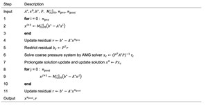
then solve the linear system Eq. 3 and update solution variables at time level n+1 until the pressure increments 𝑥𝑟 and 𝑥𝑤 and residuals 𝑏𝑟 and 𝑏𝑤 are sufficiently small. To solve each linear system in Eq. 3, we use a FGMRES iteration with a multi-stage preconditioner consisting of an ILU0 pre-smoother, a multi-scale solver and an ILU0 post-smoother summarized in Algorithm 1. The multi-stage preconditioner is formed for the reservoir equations only, and the contribution from wells is included, using an approximate Schur complement of 𝐴𝑤𝑤:

Here the parameter 𝛾 can be used to tune the approximation. Note that the right-hand side of Eq. 4 is not an approximation.

The multi-scale solver stage in the multi-stage preconditioner consists of two steps. In the first step, a set of locally computed numerical basis functions is updated, using an iterative procedure. Each basis function is the approximate fine-scale pressure response to a pressure change in a coarse block. The fine-scale pressure response is assumed to be non-zero in a small, predefined neighborhood of cells surrounding the coarse block and zero elsewhere. This neighborhood is referred to as the support region of the coarse block. In the second step, the basis functions are collected as column vectors in a prolongation matrix 𝑃 that is used to approximate the fine-scale pressure change 𝑥𝑟∈ℝ𝑁 as:

where 𝑥𝑐∈ℝ𝑀 represents the pressure change at a coarse scale and 𝑀≪𝑁. If we insert this approximation into Eq. 4 and multiply by 𝑃𝑇 to restrict both sides of Eq. 4, we get an 𝑀×𝑀 linear system for the coarse pressure changes:

which is easier to solve than the 𝑁×𝑁 linear system of Eq. 4 directly for the fine-scale pressure changes. In our implementation, we solve Eq. 7 using a single AMG V-cycle for the coarse pressure changes. Then, an approximation to the fine-scale pressure changes can be recovered, using Eq. 6.

Algorithm 1. The multi-scale, multi-stage preconditioner consists of an ILU0 pre-smoother (Steps 1 to 3), a multi-scale solver (Steps 5 to 7) and an ILU0 post-smoother (Steps 8 to 10).

COARSE GRIDS

The MsRSB algorithm takes a coarse grid with corresponding support regions as a prerequisite. In this paper, we use METIS to generate coarse grids. METIS is a general graph partitioning software package that is publicly available. METIS takes the simulation grid connectivity graph 𝑮(𝑽,𝑬) as input, where each vertex in 𝑽 is associated with a grid cell and each edge in 𝑬 represents a connection between grid cells. The output is a partition of vertices into 𝑴 disjoint sets 𝑪𝒊 such that the edge cut set is minimized. We initially define the 𝒊th support region as the cells in the corresponding coarse block, 𝑫𝒊𝟎=𝑪𝒊, and iteratively add all vertices connected to any vertex in 𝑫𝒊𝝂, i.e.:

The number of times we add connected vertices can be controlled by 𝑛𝑠𝑢𝑝𝑝 which we refer to as the support thickness. In the following, we use 𝐶 = {𝐶𝑖,𝑖=1,…,𝑀} to denote the set of coarse blocks, and 𝐷={𝐷𝑖,𝑖=1,…,𝑀} to denote the set of support regions. Figure 1 illustrates the process of the support region construction.

Fig. 1. Construction of support regions. Here, Eq. 8 is applied three times to create a support region that includes the coarse block and three concentric layers of neighbor cells. From the left, the plots show each step in the process 𝑫𝟎, 𝑫𝟏, 𝑫𝟐, and 𝑫𝟑

Restricted smooth basis functions. We briefly present the algorithm used to construct prolongation operators for the MsRSB method. The process is similar to the construction of prolongation operators for a smoothed aggregation multi-grid method (Vaněk et al. 1996): first, create a tentative piecewise constant prolongation operator, then iteratively smooth each basis function (i.e., column of 𝑷). In our commercial simulator, we have implemented the MsRSB method proposed by Møyner and Lie (2016). This multi-scale method uses a constrained Jacobi iteration to smooth the basis functions. The steps to calculate basis functions 𝑷∈𝑹𝑵×𝑴 is summarized in Algorithm 2.

Algorithm 2. Calculation of restricted smoothed basis functions.

The basis functions are updated by iterating Steps 2 to 4 until suitable convergence criteria are met. In our implementation, we measure the change in basis functions between iterations. When maximal change is less than a prescribed tolerance 𝛿, or the maximal number of iterations 𝑛𝑗𝑎𝑐𝑜𝑏𝑖 is exceeded, the iteration process stops.

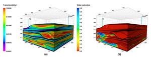
Modeling high-contrast features. From our experience with use of the multi-scale SFI method on field models, we have met several characteristics of reservoir models that degrade the performance of the multi-scale solver compared to a fine-scale AMG solver. Figure 2 shows two models that pose significant challenges for the standard MsRSB pressure solver. The first one is a field model that has a fluvial depositional system, modeled as high-permeability meandering and braided riverbeds and low-permeability barriers, Fig. 2a. The ratio of the largest to the smallest permeability is 1000:1. In addition, this model uses transmissibility multipliers between channel and non-channel rock regions to increase the contrast. The transmissibility field spans five orders of magnitude. The second example is a complex geological model with very thin layers (mm~m) used to model low-permeable shale formation, Fig. 2b.

Fig. 2. Examples of high-contrast heterogeneous reservoir models with respect to directional transmissibility fields: (a) channelized formation with high- and low-permeability zones and (b) shale thin-layered formation.

The key idea with multi-scale methods is to construct a set of prolongation operators that interpolate solutions accurately from a coarse spatial resolution to the grid resolution. In high-contrast transmissibility models, it is especially important that this flow interpolation is confined to within high-contrast boundaries to preserve large pressure differences across low-permeability structures. The new algorithm works as follows: First, it finds dominant flow directions by comparing the values of connection transmissibility in a neighborhood. Then, the algorithm emphasizes the interpolation along these dominant directions and ignores interpolation in the transverse direction if connection transmissibility is weak.

Strongly coupled neighborhood filtering. The work in this paper was inspired by Vaněk (1996), which introduced the notion of a strongly coupled neighborhood to construct aggregates for a smoothed aggregation multi-grid method. Multi-scale methods can be viewed as two-level versions of AMG with aggressive coarsening. Therefore, we follow the approach of smoothed aggregation multi-grid methods to define a coarsening strategy, using strongly coupled neighborhoods. Vaněk defines a strongly coupled neighborhood of vertex 𝒊 as:

This definition is suitable for elliptic problems. Here, we need to change the transmissibility values 𝑡𝑖𝑖 and 𝑡𝑗𝑗 in Eq. 9 to ensure diagonal dominance and zero row sum:

The definition of a strong neighborhood is symmetric: If 𝑗 is strongly connected to 𝑖, then 𝑖 is strongly connected to 𝑗, i.e., if 𝑗∈𝑁𝑖(𝜀), then 𝑖∈𝑁𝑗(𝜀). This can be used to partition the edges (𝑖𝑗) into weak ones and strong ones that satisfy this condition. It can also be used to define an edge filter that keeps only the strong edges:

The threshold 0≤𝜀≤1 determines what is considered to be a strong edge (or connection). If 𝜀=0, no edges are removed and 𝐸𝐹=𝐸, while if 𝜀=1, all edges are removed and 𝐸𝐹=∅. We discuss the sensitivity of the filtering algorithm for other choices for 𝜀 in a later section.

The new algorithm consists of four steps summarized in Algorithm 3. We only compute Steps 1-3 once at the beginning of simulation and update MsRSB basis functions, using Step 4 at the start of every nonlinear pressure iteration. All algorithm steps are implemented, using high-performance parallel computations.

Algorithm 3. Steps to compute the multi-scale prolongation operator in f-MsRSB.

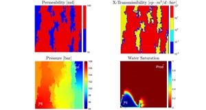
MODEL 1: Synthetic two-dimensional model. To illustrate the issue with high-contrast features, we start with a two-dimensional, two-phase immiscible and incompressible simulation case with two sets of boundary conditions, Fig. 3. For simplicity, the fluids have unit viscosity ratio and linear relative permeabilities. One case has pressure boundary conditions on the west and east domain boundaries (Model 1a) with a pressure difference of 100 bars.

The other case has the same pressure difference boundary conditions on the north and south domain boundaries (Model 1b). For the case with a west-east pressure boundary condition, due to the low-permeability region of 0.001 md in the middle of the background permeability of 100 md, Fig. 3a. The simulated pressure field is highly affected across the low transmissible rock region, showing high-pressure values in the left side of the domain and low-pressure values in the right side of the domain in Fig. 3b. This is because the dominant flow in the 𝒙 direction is perpendicular to the uniform transmissibility field in the 𝒚 direction. While for the case with north-south pressure boundary condition, the dominant flow in the 𝒚 direction is aligned with the uniform transmissibility field in the 𝒚 direction. Here, the simulated pressure field is smooth, and it does not exhibit a sharp contrast profile, Fig. 3c.

Fig. 3. Permeability field with low-permeability feature (left), pressure field for Model 1a with west-east pressure boundary conditions (middle), and pressure field for Model 1b with north-south pressure boundary conditions (right).

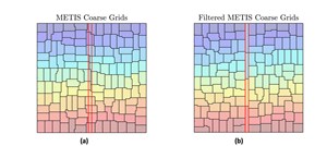
Figure 4 shows coarse grids for Model 1. Fig. 4a shows the standard approach to generate coarse grids, which is to pass 𝐺(𝑉,𝐸) with original edges to METIS. This coarse grid contains coarse blocks that cross the boundary between high- and low-permeability zones. By passing the graph 𝐺(𝑉,𝐸𝐹) with only strong edges to METIS, we ensure that coarse gridblock boundaries are aligned with the boundary between low- and high-permeability zones, as shown in the righthand plot, Fig. 4b.

Fig. 4. Example (a) shows METIS partitioning with the original connectivity graph 𝑮(𝑽,𝑬) and (b) shows METIS partitioning using the filtered connectivity graph 𝑮(𝑽,𝑬𝑭). The coarse grid boundaries are in black, and the red lines delineate boundaries between high- and low-permeability regions. Coloring is based on numbering coarse gridblocks.

MODEL 2: Synthetic high-contrast heterogeneous model. Now, the general applicability and robustness of the new algorithm is tested on a synthetic high-contrast heterogeneous model using multipoint geostatistics with Stanford Geostatistical Modeling Software (SGeMS). The permeability field is generated with a long correlation length and an orientation designed to model two different rock regions. To make the model resemble the model shown in Fig. 2a, we assigned transmissibility multipliers of 1.0e-8 to connections between the two rock regions. The resulting model is shown in Fig. 5. Rock and fluid properties are the same as used in Model 1.

Fig. 5. High-contrast heterogeneous simulation case with one injector and one producer.

FIELD-SCALE MODELS

The following simulation performance evaluations are conducted on our in-house cluster, which consists of dual-socket, multi-core machines with an AMD EPYC™ 7532 processor running at 1.8 to 2.4 GHz CPU, with each machine having 1 TB of memory. We compare the CPU times for the fine-scale AMG pressure solver (Fine-scale AMG), the multi-scale pressure solver with the full connectivity graph (MsRSB), and the multi-scale pressure solver with the filtered connectivity graph (f-MsRSB). The settings for the SFI method are configured exactly the same to evaluate the impact of different pressure solvers only.

MODEL 3: Synthetic waterflood model. The first field-scale performance test is a synthetic waterflood model. This is a high-contrast heterogeneous fluvial-channel reservoir, Fig. 6. The contrast in permeability between channel and non-channel regions is three orders of magnitude, from 1 to 1,500 md, and contrast between channel and non-channel regions is increased by using a transmissibility multiplier of 1.0e-5. Altogether, the transmissibility values span five orders of magnitude. The field is produced with 30 wells—16 producers and 14 water injectors—which are completed in high-quality oil and water zones, respectively. The wells open sequentially, according to a drilling schedule, and operate for 58 years.

Fig. 6. Permeability field in md (left) and transmissibility filed in the I-direction in the layer 74 section (right).

The model has 240×192×100 cells with over 2.3 million active cells. Figure 7 shows the pressure field (left) and saturation field in a single layer (right) at the end of the simulation. The pressure and saturation fields are strongly affected by the contrast in the transmissibility field. Pressure in the channel is depleted with the connected producers and water preferential flooding through high-permeability regions along channels. The production scenario is simulated on 48 cores using the three solver options.

MODEL 4: Computational stratigraphy reservoir model. Next, we run a synthetic model created using Chevron’s Computational Stratigraphy (CompStrat) modeling framework. CompStrat is a physics-based approach that can accurately predict and model reservoir structure, facies and permeability by connecting to fundamental sedimentary processes through computational modeling. In particular, the method captures the details of stratigraphic flow barriers, which enables accurate predictions of flow performance.

The 3D model has over 4.4 million active cells shown in Fig. 7. The grid has 40 cells in lateral directions, each cell having a size of about 20 m. At the same time, we have 2,800 cells in the vertical direction, while the thickness of the reservoir is only about 18 m. This results in the cell average vertical size of 6 mm, and the resulting average cell aspect ratio of more than 3,000. Moreover, highly heterogenous permeability results in a huge transmissibility contrast, with the maximum vertical transmissibility going up to 1.0e7 [𝑐𝑃 ∙ 𝑚3/𝑑 ∙ 𝑏𝑎𝑟], while the lateral values are about 1 [𝑐𝑃 ∙ 𝑚3/𝑑 ∙ 𝑏𝑎𝑟]. We simulate a water-flooding scenario with one producer and one injector where initial oil saturation is 0.8 and the simulation period is 1,522 days. For this case, the transport solver uses the hybrid upwind discretization for viscous and gravity flows to stabilize the nonlinear convergence and prevent upwind flip-flopping. We have simulated this model with the three solver options, using 128 cores in our in-house cluster.

Fig. 7. Pressure field in bar (left) and water saturation (right) in the Layer 45 section at the end of simulation.

For this model, the multi-scale pressure solver fails without using the filtering algorithm: the pressure solution diverges from the fully implicit reference solution and cuts the timestep size to prohibitively small values, and the results are not shown in the following comparisons. Conversely, in terms of the field responses, the new filtering algorithm leads to robust performance and perfect agreement with both the FI run and the SFI run with fine-scale AMG pressure solver, Fig. 8.

Fig. 8. Computational stratigraphy reservoir model showing (a) the transmissibility field in the J direction and (b) the water saturation profile at the end of the simulation.

MODEL 5: Field model with high-contrast channelized reservoir. Finally, we use a real three-phase field model from a client. For the confidentiality of the data, we are unable to share many details about the model. The zoomed transmissibility field, shown in Fig. 2a, gives an impression of the heterogeneity of this model. The transmissibility field spans five orders of magnitude with different rock regions and channelized reservoir geology in a fluvial depositional environment.

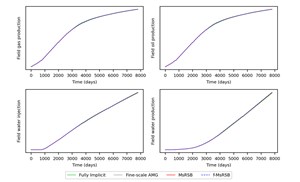
Moreover, the model is structurally complex, like Danish pastry, with isolated layers and inactive cells due to pinchouts, to honor the field reservoir geological characterization. The total number of active cells is more than 1.3 million. We have simulated this model with the three solver options, using 48 cores in our in-house cluster. Figure 9 shows the field simulation responses, and all runs are in excellent agreement with responses of the reference FI run. Figure 10 displays iteration numbers and total CPU time for the three solver options.

Fig. 9. Results for the fully implicit method (green solid line) and for the sequential fully implicit method with the fine-scale AMG pressure solver (black dotted line), the standard MsRSB pressure solver (red solid line), and the f-MsRSB pressure solver (blue dashed line).

Fig. 10. Results for the sequential fully implicit method with the fine-scale AMG pressure solver (black dotted line), the standard MsRSB pressure solver (red solid line), and the f-MsRSB pressure solver (blue dashed line). The total CPU time for the fully implicit run (green solid line) has been added for reference.

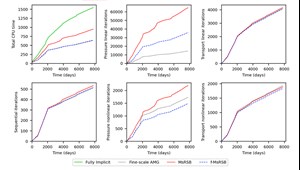
In this case, linear and nonlinear iterations and CPU times are summarized as follows. The f-MsRSB algorithm reduced the pressure solver linear iterations by 44% and nonlinear solver iterations by 32%, in comparison with standard MsRSB run. Consistently with Model 3 and Model 4 results, the per-iteration linear solver CPU time is smaller for the multi-scale with filtering algorithm than for the fine-scale AMG pressure solver, and the total CPU time of the multi-scale pressure solver with filtering algorithm is comparable to that of the fine-scale AMG pressure solver.

CONCLUSIONS

For high-contrast heterogeneous reservoirs, we find that the poor linear-solver convergence of the multi-scale pressure solver is caused by interpolation errors that originate from poorly calculated basis functions. This reduces the effectiveness of the MsRSB preconditioner and even creates artifacts in the intermediate pressure solutions that require many ILU0 iterations to smooth out.

The new algorithm defines a strongly coupled neighborhood by comparing the transmissibility of connections to a grid cell. To deal with high contrasts in the transmissibility field, the new algorithm filters the connections that are significantly weaker than average in a neighborhood. The filtering prevents the interpolation error that occurs in the MsRSB method when coarse gridblocks and support regions cross low-transmissibility features. This improves basis function computation in the MsRSB method and the effectiveness of the MsRSB preconditioner.

We have tested the new algorithm on synthetic and field-scale models and demonstrated that this has improved simulation performance. The improvement was attributed in part to fewer iterations in both the linear and nonlinear solver, and in part to better per-iteration computational efficiency. We have evaluated the practical efficiency comparisons of the standard fine-scale AMG pressure solver and the multi-scale solver in our simulator, and we have discussed the trade-offs between convergence speed and computation cost.

NOMENCLATURE

𝜀= filter tolerance

𝜈= iteration level

𝑆= Jacobi smoothing matrix

𝑑𝑖𝑎𝑔(𝐴) = diagonal of matrix 𝐴

𝑑𝑖𝑎𝑔 (𝑣) = matrix with elements of the vector 𝑣 on the diagonal

ACKNOWLEDGMENTS

This article contains excerpts from a technical paper, “Strongly coupled prolongation in multiscale pressure solver for high-contrast heterogeneous reservoir simulation,” SPE paper 212229-MS, presented at the SPE Reservoir Simulation Conference held in Galveston, Texas, March 28–30, 2023. The work was supported by the SLB Chevron INTERSECT Alignment committee and builds on a decade of development by scientists in Houston and Oslo, in addition to commercialization engineers in Abingdon, UK.