Exploration Technology

Seismic interpretation of water saturation based on reflectivity transforms

Two rock-property transforms combined with an AVO thin-bed response allow for improved water-saturation estimation.

Fred Hilterman, Zhengyun Zhou and Haitao Ren, Center for Applied Geosciences and Energy, University of Houston

A seismic interpretation technique is introduced that combines near- and far-angle amplitude maps to yield a map whose values are estimates of NI. The NI difference between the prospect and its equivalent down-dip wet reservoir leads to the prediction of the pore fluid and water saturation (S_W).

The two, new rock-property relationships are the Lithology and Pore-Fluid Transforms. The first relates the lithology of the sand reservoir and its encasing shale to the slope that is derived from Amplitude-Versus-Offset (AVO) analysis. The second transform relates the AVO-derived intercept (NI) to the pore fluid. By combining the lithology transform with the AVO thin-bed response, NI_HYDRO values for the upper interface of the reservoir are predicted, regardless of the thickness, porosity, cementation, encasing shale properties, etc.

The prospect is tested for different S_W. Each S_W test requires two maps. The first map, which is derived from a lithology transform with a specific S_W, yields an estimate of NI_HYDRO across the prospect, while the second map, using a wet lithology transform, yields an estimate of NI_WET across the assumed equivalent sand that is down-dip and wet.

The tests with different S_W are stopped when the difference between the prospect NI_HYDRO and the down-dip wet NI_WET equates to the pore-fluid transform prediction for the same S_W. To reiterate, the interpretation compares NI values at two different map locations, one at the prospect and the other at a down-dip location. A field example across a Tertiary reservoir in the Gulf of Mexico illustrates the technique.

INTRODUCTION

In the Gulf of Mexico, gas saturation is always an important seismic interpretation issue. The reason is that a small amount of gas usually lowers the reservoir’s P-wave velocity dramatically and, as gas saturation increases, the P-wave velocity does not change significantly. In unconsolidated sediments, the seismic amplitude change from a gas reservoir (S_W=30%) is large compared to the reflection from a wet reservoir. The large amplitude change is recognized as a diagnostic indicator of hydrocarbons.

However, a large difference in amplitude also exists for fizz (S_W=90%) reservoirs. Hence, fizz and gas reservoirs are often indistinguishable using seismic amplitude. Numerous interpretation techniques, including AVO, have been suggested to resolve the S_W dilemma. To understand the magnitude of the differences between fizz and gas reflections, their reflection properties will be reviewed.

The Zoeppritz AVO curves for three different pore fluids in the same reservoir are illustrated in Fig. 1a.¹ When going from wet to fizz saturation, 93% of the NI difference comes from the P-wave velocity change. While going from fizz to gas, 97% of the NI difference comes from the pore-fluid density change. This example illustrates that if sand reservoirs in the area maintain constant porosity, lithology, thickness and encasing shale properties, then the seismic near-trace amplitudes will differentiate fizz from a gas reservoir.

Fig. 1. Zoeppritz AVO curves. a) SW variations for sand with j=31%, b) fizz (SW=90%) and gas (SW=30%) for two different porosity sands.

However, Fig. 1b illustrates² that a reservoir with 34% porosity (S_W =90%) has, for all practical purposes, the same AVO response as the previous 31% porosity reservoir (S_W =30%). Thus, using only the seismic AVO response across a reservoir will not differentiate fizz from a gas reservoir unless some restrictions, such as sand porosity, are known or assumed.

The distinction between fizz and gas reservoirs is illustrated again with the AVO synthetics shown in Fig. 2. Down-dip wet synthetics and their corresponding hydrocarbon-saturated synthetics are shown for three different reservoirs labeled (a), (b) and (c). In the lower portion, only reservoir (a) is gas saturated, the others have fizz. However, the AVO synthetics for the reservoirs represented by (b) and (c) are very similar to the gas synthetic in (a). The reservoir corresponding to the (b) synthetic has an increase in porosity over (a) while the reservoir for the (c) synthetic has encasing shale that is harder than the others.

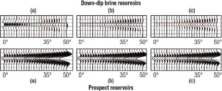Fig. 2. AVO synthetics for three different reservoir models. Top row are down-dip brine-saturated reservoirs. Corresponding up-dip prospects (bottom row) are (a) gas, j=30%, (b) fizz, j=33% and (c) fizz, j=30%, with hard-encasing shale, all of which are similar. The AVO response of the down-dip wet sand (a) helps differentiate fizz from gas in the corresponding up-dip gas reservoir.

In short, Figs. 1 and 2 illustrate that if the reservoir sand changes porosity, cementation, lithology ... or the encasing shale properties become harder or softer, etc. ..., then, the AVO amplitudes of the prospect will NOT distinguish fizz from gas even if the seismic amplitude is calibrated to a local well. However, Fig. 2 shows that the AVO response of the down-dip wet sand will help differentiate fizz from the up-dip gas reservoirs. That is, S_W differentiation is possible by comparing the seismic response at the down-dip portion to the seismic response at the prospect. To apply this observation, the amplitude differences need to be calibrated to borehole data.³

ROCK-PROPERTY TRANSFORMS

Insight on how to quantify the amplitude relationships observed in Figs. 1 and 2 comes from Hendrickson.⁴ He mentions that the AVO slope “... is dominated by the lithology,” while the “pore-fluid effects are expressed primarily by the normal-incident P-wave response.” In this respect, the objectives of the rock-property transforms are: 1) to quantify various NI_HYDRO in terms of NI_WET, and 2) to quantify the far-angle amplitude (RC(30°)_SATURANT) in terms of the near-angle amplitude (RC(0°)_SATURANT) for various pore-fluid saturations. In essence, pore-fluid and lithology transforms are needed.

For this study, the lithology and pore-fluid transforms were derived from the TILE2 area of a database provided by Geophysical Development Corp. Rock properties from 320 wells in the northern West Cameron and High Island areas were included. Velocity and density values at 200-ft intervals were extracted for wet-sand reservoirs and their encasing shale from depths of 800 to 18,000 ft.

Statistics from 16,605 intervals were available. Limiting the depth range to that of the prospect (7,100-9,100 ft), and requiring both velocity and density values for sand and shale, reduces the number of intervals to 660. Fluid substitutions for fizz (S_W=90%) and gas (S_W=30%) were conducted using fluid properties from Batzle and Wang⁵ and S-wave estimations from Greenberg and Castagna.⁶

The resulting pore-fluid and lithology transforms are shown in Fig. 3. With the pore-fluid transforms in (a), NI_FIZZ or NI_GAS can be predicted once NI_WET is known. The slope values for the pore-fluid transforms in (a) are essentially the same, indicating that (NI_WET – NI_GAS) is constant in the study area. Likewise, the (NI_WET – NI_FIZZ) difference is also constant.

Fig. 3. Rock-property transforms developed for study area.

Normally, the NI_HYDRO from the top interface of a reservoir and the NI_WET from the down-dip are unknown, thus constraining the possible application of the Pore-Fluid Transforms. However, many mathematical models relate seismic amplitude to NI by an unknown scale factor (such as =K 3 NI). Thus, A/B measurements are often made where B is the wet down-dip seismic amplitude and A is the prospect seismic amplitude. Then, the seismic A/B equates to NI_HYDRO/ NI_WET.

However, from Fig. 3a, NI_GAS/ NI_WET = -0.092/ NI_WET + 1.17. There is a problem in that the A/B measurement from seismic can’t be compared to the NI_GAS/ NI_WET from the pore-fluid transform because NI_WET is unknown. Zhou, et al.² gave the solution to this dilemma through a simple application of the Lithology Transform to the AVO thin-bed response.

MATHEMATICAL MODEL

The technique uses the mathematical expression for a thin-bed as shown in Fig. 4.⁷ The seismic amplitude, A(q), contains a multiplicative factor, k, that one assumes is constant for a 3D seismic survey, at least for a given depth zone. This means no automatic gain corrections (AGC) were applied during processing.

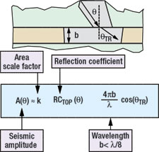Fig. 4. Seismic model for a thin bed reflection.

The seismic amplitude at the incident angle q is related to the Zoeppritz reflection coefficient from the top interface of the thin bed, RC_TOP(q). The Widess thin-bed scalar is included and, thus, limits this particular mathematical model to reservoir beds that are thinner than 1/8th wavelength. For most applications, beds thinner than 40 ft satisfy this loose constraint. For beds thicker than this constraint, the mathematical model is easily adjusted. Finally, the cosine term is a function of the propagation angle in the reservoir, but the incident angle is a good approximation.

The next step is to illustrate how the near- and far-angle stacks can be combined to yield NI. The first equation in Fig. 5 is the general expression of a lithology transform. The variables a₀ and a₁ have specific values depending on the pore fluid specified.

Fig. 5. NI in terms of seismic near- , A(0°), and far-angle amplitudes, A(30°).

Line 2 is an algebraic manipulation of line 1. Line 3 has three terms on the right side. The first term states that NI is equivalent to RC(0°) if the second and third terms are each equal to one, as they are. In the numerator of line 3, the term (RC(0°) × k × 4pb/ l) is equivalent to the seismic amplitude A(0°) as given by the thin-bed model in Fig. 4. The same logic is applied to the denominator to yield the expression in line 4. In line 4, the NI value is expressed in terms of the seismic near-angle, A(0°), and far-angle, A(30°), amplitudes, along with a₀ and a₁ that are associated with the specified lithology transform.

FIELD EXAMPLE

The near- and far-angle horizon maps in Fig. 6 cover approximately 9 sq mi (one federal offshore block). The target sand horizon is at a depth of about 8,000 ft and has normal pore pressure. The blue outlines on the near- and far-angle maps represent a known gas field that we will assume is the prospect where an estimate of S_W is desired. The area to the southeast of the prospect is most likely the same formation, but is wet. As a first step, the assumed wet area to the southeast is converted to NI values that represent NI_WET. For the time being, the pore-fluid of the prospect is unknown.

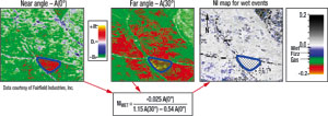Fig. 6. Transforming near- and far-angle maps into brine-saturated NI values. Click image for enlarged view

The near- and far-angle maps are then combined as shown by the NI_WET lithology transform on the bottom in Fig. 6. This lithology transform for wet zones will yield “true” NI values on the map where the formation is wet. Thus, the prospect is covered to indicate that this area will not have its true NI values because a wet lithology transform was applied, and it is assumed that the prospect contains hydrocarbons of unknown S_W.

The two amplitude color bars indicate the range of values for the seismic horizon maps and the NI wet map. Only, the rightmost color bar has scales that are representative of reflection coefficients. Superposed on this color bar are the expected NI values for wet, fizz and gas saturations taken from a nearby well. In general, the NI horizon map is in agreement with the expected values from the nearby well-log calibration. In the upper right of the NI horizon map is a small triangular shaped area that has NI values that vary significantly. This is a zone that apparently doesn’t conform to our assumption of a thin-bed wet sand.

The NI map for the wet areas is shown again in Fig. 7, along with the pore-fluid transform that converts NI_WET to NI_GAS values. Application of the transform yields the NI_GAS map. As a check, the color bar indicates that the portion of the map down-dip from the prospect now has values representative of NI_GAS. In a similar fashion, the fizz pore-fluid transform could have been applied, thus changing the background NI_WET values to NI_FIZZ.

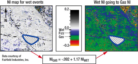Fig. 7. Converting down-dip brine NI values into gas-saturated NI values.

A summary of the interpretation technique is shown in Fig. 8. The map shown in (a) is the previous lithology transform for the wet areas. Once again, the prospect is shaded out because the prospect is assumed not to be wet. Map (b) represents a lithology transform assuming the prospect is fizz saturated, while map (c) is a lithology transform assuming the prospect is gas saturated. Map (d) is a wet-to-fizz pore-fluid transform of the wet NI map in (a). Likewise, map (e) is a wet-to-gas pore-fluid transform of the wet NI map in (a).

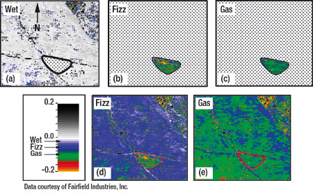Fig. 8. Comparing down-dip NI values for various SW fluid substitutions to respective lithology transforms at prospect.

The final analysis comes when the prospect NI values are transferred from the upper maps, (b) and (c), into their respective locations in the lower maps, (d) and (e). This has already been done in Fig. 8. The question remains for Figs. 8d and 8e, “Do the down-dip NI values in (d) or (e) best match its prospect NI values?” For this field example, the gas-saturation scenario in (e) is the better match. And, as mentioned earlier, this is a gas field.

A FEW POINTS

Because this is a relatively new interpretation technique, several points are addressed.

• The seismic horizon maps are assumed to represent a thin-bed sand formation.
• The prospect is assumed to have a down-dip wet portion that has the same lithology as the prospect. If the prospect is a stratigraphic trap or is too structurally complex to find the down-dip portion, then this technique is not applicable. If the prospect preserved porosity, because of its hydrocarbon saturation, while the down-dip portion didn’t, then this technique is not applicable.
• The thickness of the down-dip portion does not have to be the same as the prospect thickness.
• The phase of the seismic wavelet is not critical as long as phase changes are recognized in the event picking of the target horizon. That is, if the wet portion is opposite polarity to the prospect, then the seismic mapped horizons must honor this in their picked amplitudes.
• Relative gain is maintained during processing.
• Calibration of the far-angle to the near-angle stack is easily accomplished by multiplying the far-angle map by a constant, run a wet lithology transform, and then compare the resulting NI_WET at a known well location.
• Pore-fluid and lithology transforms are locally derived for the target depth.

CONCLUSIONS

Two rock-property transforms are paramount in developing the new interpretation technique for estimating pore fluid and S_W. The first is the pore-fluid transform that establishes the difference between NI_WET and NI_HYDRO. In this study area, NI_WET – NI_GAS is about 0.09 while NI_WET – NI_FIZZ is only 0.06. The NI difference discriminates fizz from gas. However, to apply this information, the seismic amplitudes are first converted to NI values. This is the function of the Lithology Transform.

The conversion of the prospect seismic amplitudes to NI requires a different lithology transform from the one applied to the seismic amplitudes across the wet areas. Each lithology transform is associated with a specific S_W. After applying a specific S_W lithology transform to the prospect, the difference NI_PROSPECT – NI_WET is compared to the corresponding difference derived from the pore-fluid transform for the same S_W. If equal, an estimate of S_W is determined.

There are many avenues that need to be investigated for this new interpretation technique. Though not mentioned, it has been numerically determined that the technique is accurate for thin beds that have velocity/ density gradients if the result is considered as a Backus-averaged effective medium. A few numeric sensitivity tests with regard to S_W have been applied, but the more important issue of verifying variations of S_W with field data is still being investigated.

The small theoretical difference between NI_GAS and NI_FIZZ cannot be ignored; it will come into question when the seismic S/N ratio is not as good as the data used in this study. Also, the astute eye will note that the color bar in Fig. 8 was carefully chosen to separate wet, fizz and gas saturations with distinctly different colors. This privilege is normally not available. 

ACKNOWLEDGEMENTS

Two companies provided data and allowed us to show the results: Fairfield Industries for 3D AVO seismic data and Geophysical Development Corp. for the rock-property database. Support for this study comes from the sponsors of the Reservoir Quantification Laboratory at the University of Houston. Portions of this work were prepared with the partial support of DOE grant, DE-F26-04NT15503. However, any opinions, findings, conclusions or recommendations expressed herein are those of the authors and do not necessarily reflect the views of DOE.

LITERATURE CITED

  ¹ Hilterman, F. J. and L. Liang, “Linking rock-property trends and AVO equations to GOM deep-water reservoirs,” 73rd Ann. Internat. Mtg., Soc. Expl. Geophys., Expanded Abstracts, pp. 211-214, 2003.
  ² Zhou, Z., Hilterman, F., Ren, H., and M. Kumar, “Water-saturation estimation from seismic and rock-property trends,” 75th Ann. Internat. Mtg., Soc. Expl. Geophys., Expanded Abstracts, 258-261, 2005.
  ³ Ren, H., Hilterman, F., Zhou, Z., and M. Kumar, “Seismic rock-property transforms for estimating lithology and pore fluid content,” AAPG Ann. Mtg., 2006.
  ⁴ Hendrickson, J.S., “Stacked,” Geophys. Prosp., Vol. 47, pp. 663-706, 1999.
  ⁵ Batzle, M. and Z. Wang, “Seismic properties of fluids,” Geophysics, Vol. 7, pp. 1396-1408, 1992.
  ⁶ Greenberg, M.L. and J. P. Castagna, “Shear-wave estimation in porous rocks: Theoretical formulation, preliminary verification and applications,” Geophys. Prosp., Vol. 40, pp. 195-210.
  ⁷ Lin, T. L. and R. Phair, “AVO Tuning,” 63rd Ann. Internat. Mtg., Soc. Expl. Geophys., Expanded Abstracts, pp. 727-730, 1993.

THE AUTHORS
	Fred J. Hilterman holds the Margaret Sheriff Chair in Geophysics at the University of Houston. He received a geophysical engineering degree and PhD in geophysics from the Colorado School of Mines. He worked for Mobil from1963 to 1973 before joining the University of Houston. At UH, Hilterman co-founded the Seismic Acoustics Laboratory (SAL) in 1976. He co-founded Geophysical Development Corp. in 1981 and was VP of Development until 2003, when he rejoined UH.
	Zhengyun Zhou is currently a PhD student of geophysics at the University of Houston. She is also a research assistant in the Reservoir Quantification Lab (RQL). Her research focuses on water saturation estimation and long-offset migration. She received a BE degree (1999) and an ME degree (2002) from Ocean University of China. Before becoming a PhD student, she worked as a research geophysicist in Geophysical Information Technology Lab, Ocean University of China.
	Haitao Ren is currently a PhD student of Geophysics in University of Houston. He is also a research assistant in the Reservoir Quantification Lab (RQL). His research focuses on rock physics and seismic physical modeling. He received a BS degree in geology (2001) and an ME degree in Petrophysics (2004) from University of Petroleum, China.