Production Technology

Predicting production performance using a simplified model

Neither hyperbolic nor exponential models fully explain decline. So, why not simply combine them?

Khaled Abdel Fattah, Kh. A., King Saud University, Saudi Arabia

One of the most important tasks of the petroleum engineer is predicting the amount of oil and gas that will be recovered from a reservoir. Choosing the methodology is critical for accurate forecasts that are, in turn, vital for sound managerial planning. Decline curves are widely used to convey information about past production performance and to forecast future performance and reserves. A new model for decline curve analysis has been developed. The new model uses an exponential decline to extrapolate a hyperbolic decline to prevent unrealistically long lifetime and reserve estimates.

INTRODUCTION

Management needs to reduce the risks associated with decision making, and one of the ways in which this can be done is by anticipating future well performance more clearly. Extrapolation of production history has long been considered the most accurate and defendable method of estimating remaining recoverable reserve from a well and, in turn, a reservoir. The technique for relating production to time is known as decline curve analysis, and is a very useful tool for estimating future production. The decline curve is often used to determine the economic limit of a well, estimating the remaining reserves, and forecasting the present worth of the oil and gas reserves in the future.^1–5

Three types of decline curves are considered, although only two of three techniques, namely, exponential and hyperbolic, commonly occur in reservoirs. The hyperbolic decline model predicts a longer well life than is predicted by the exponential decline model. Also, the exponential forecast provides the lowest estimate of recoverable reserves. Experienced evaluators avoid extrapolating hyperbolic declines over long time periods, because they frequently result in unrealistically high reserve and value estimates.^6–8 Many wells follow the trend toward an exponential decline in their later life. Long and Davis⁹ developed a log-rate-versus-time overlay to cope with this problem. This type of curve matching has some disadvantages, mainly due to the non-uniqueness problem in determining the correct type of curve to use. Robertson¹⁰ developed a production rate equation that is hyperbolic initially but asymptotically exponential with time. He introduced a dimensionless constant; its value ranges from 0 to 1 and is related to the abandonment pressure, and the rock and fluid properties.

One of the main difficulties is to find the transition point between the hyperbolic and exponential decline curves, that is, the endpoint of hyperbolic decline and the starting point of exponential decline. Long and Davis,⁹ and Robertson¹⁰ ignored determining the precise transition point between the hyperbolic and exponential declines; they assumed the exponential decline rate was known based on the experience with analogous wells or experience with particular reservoirs. In this study, however, a distinct technique is formulated to find this exponential decline rate and determine the transition point of transferring the hyperbolic to exponential decline curve.

DECLINE CURVE ANALYSIS

Exponential decline curve. The most commonly used decline curve is exponential because of its simplicity. Equations of exponential decline are given by:

(1)

The above equation has two constants, the initial production rate, q_o, and the exponential decline rate, D, which is constant for all time. Together, they yield the cumulative production:

(2)

Hyperbolic decline curve. Hyperbolic decline occurs when the decline rate is no longer constant. Compared to exponential decline, the following two hyperbolic decline-curve equations estimate a longer production life of the well.¹¹

		(3)
		(4)

As can be seen in Eq. 3 the production rate, q, is related to the initial production rate, q_o, time, t, and the decline rate, D, at which production decline occurs. Eq. 3 is used primarily for the purpose of forecasting future production rates. Thus, one normally wants to extract the parameters of the rate equation by fitting it to actual production records for a well. The remaining life of the well to abandonment can be calculated by this equation. In addition, the integration of Eq. 3 with time gives the cumulative production shown in Eq. 4. From Eq. 4 one may calculate the amount of reserves in the reservoir.^12–16

PROPOSED METHOD

The hyperbolic curve frequently yields an unrealistically high reserve estimate and lifetime because the curve continually flattens with time. To compensate for this problem, a solution has been implemented that limits the minimum decline rate value. This paper develops a simple technique for evaluating production data by decline curves. Taking the derivative of Eq. 3 with respect to time, results in:

(5)

Eq. 5 may be arranged:

(6)

From the definition of the hyperbolic decline curve,^17–22 the value of decline rate, D, at time, t, can be determined from the following equations:

		(7)
		(8)
		(9)

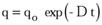
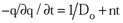
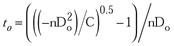
By differentiating this equation to determine the time, t_o, as shown in the Fig. 1, at which one must change the forecast from hyperbolic to exponential decline.

Fig. 1. Typical plot of oil production rate vs. time.

		(10)
		(11)

¶D / ¶t is the rate of change of decline rate with time; which is constant, i.e., C. C should close to zero where the decline rate of exponential decline is constant for all time, to match the transition point to transfer from hyperbolic to exponential decline. If the transition point occurs at t_o, then from Eq. 11, t_o can be expressed as:

(12)

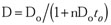
From this time value, t_o, we can determine the corresponding exponential decline rate, D, which will be constant over the next time period to the economic limit by substituting t_o in Eq. 9:

(13)

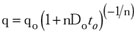
And, the initial exponential production rate may be obtained by substituting t_o in Eq. 3: 

(14)

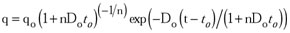
A production rate in the exponential decline segment can be expressed by expanding Eq. 1 as follows:

(15)

Thus, the combined hyperbolic and exponential production decline equation can be expressed as follows:

Hyperbolic decline segment

(16)

Exponential decline segment

(17)

PRODUCTION FORECAST EXAMPLE

Field case data⁹ are used to illustrate the new technique. The example has coefficients of q_o= 850 bbl/month, n=1.7 and D_o= 0.006873/month for the hyperbolic forecast segment, and is used to illustrate the production forecast and reserve estimation using the combinations of decline Eqs. 3 and 15. Summarized below is the procedure used to perform the production forecast:

1. Identify a rate-time relationship from fitting production history using Eq. 3. 
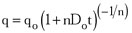
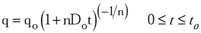
2. Identify the time, t_o, at which the forecast should be changed from a hyperbolic to an exponential curve. Fig. 2 shows the relation between the constant, C, and t_o, for the field case, and from which one can choose a reasonable value of C. In this case, t_o is found equal to 28.7 months, by using Eq. 12, with the constant C equal to – 4.5^–05.
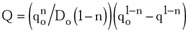
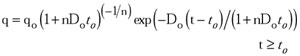
3. Determine the hyperbolic decline rate at different time values from Eq. 9, with D_o= 0.006873 and n=1.7.
4. Plot the hyperbolic decline rate predicted versus time as shown in Fig. 3.
5. Determine an initial production rate for the exponential decline, 717 bbl/month, by substituting in Eq. 14 with q_o= 850 bbl/month, n=1.7, t=28.7 months and D_o= 0.006873/month.
6. Determine an exponential decline rate, 0.005145 /month, by substituting in Eq.13, with n=1.7, t_o =28.7 months and D_o=0.006873 /month.
7. Perform the production forecast for an exponential decline curve at any time, t, greater than t_o by using Eq.17 with q_o= 850 bbl/month, n=1.7, t_o =28.7 months and D_o= 0.006873 /month.
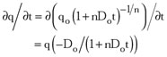
8. Plot the oil production rate predicted by both hyperbolic and exponential decline curves versus time as shown in Fig. 4.
9. Determine the reserves to be produced during the hyperbolic segment by using Eq. 4, which equals to 22,373 bbl, during the first segment of 28.7 months before it changes to an exponential decline curve, with q_o= 850 bbl/month, n=1.7, t_o = 28.7 months, D_o= 0.006873 /month. 
10. With the economic monthly rate input, the model calculated the number of months until economic depletion occurs and what the total economic reserves are.
11. If the economic production rate, q_e, is equal to 100 bbl/month, determine the reserves to be produced during the exponential segment by using Eq. 2, which is equal to 119,900 bbl with q_o= 717 bbl/month, q_e=100 bbl/month and D = 0.005145/month, from the initial decline of an exponential curve until the economic production rate.
12. Determine the total reserves to be produced during the hyperbolic and exponential segments, which is equal to 142,273 bbl.
13. If we use the hyperbolic decline curve only to fit the production rate versus time, the total reserves will be equal to 613,595 bbl for the time period, which equals to 3,168.5 months (264 years!), which corresponds from the initial production until the economic production limit, 100 bbl/month, as shown in Fig. 5.

Fig. 2. Relationship between the C constant and to.

Fig. 3. Decline rate predicted by hyperbolic decline model vs. time.

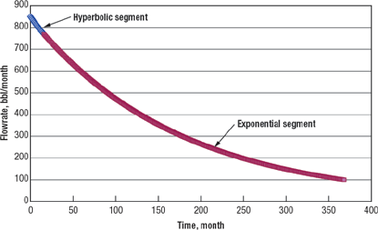Fig. 4. Oil production rate predicted by both hyperbolic and exponential decline model vs. time.

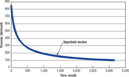Fig. 5. Oil production rate predicted by hyperbolic decline model vs. time.

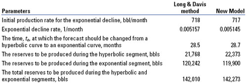
The results have been compared with the results of Long and Davis and shown in Table 1. It is clearly seen that the proposed model provides similar results.⁹

TABLE 1. Comparison of the results between Long & Davis and the New Model.

CONCLUSIONS

A new model for the production performance of reservoirs was developed. The model uses an exponential decline to extrapolate a hyperbolic decline to prevent unrealistically long lifetime and reserve estimates.

The model includes a deterministic approach to estimate the time at which one must use an exponential decline to extrapolate a hyperbolic decline. The model introduces a simple method to obtain the point where the decline is expected to hold and follow an exponential decline. One can easily calculate reserves for the separate hyperbolic and exponential decline segments, and add them together to estimate the total remaining reserves.

The proposed model is simple compared to the models available in the literature, and provides similar results while saving significant time and efforts. In other words, this model is very handy and easy to use, especially for routine industry tasks. 

LITERATURE CITED

  ¹ DeSorcy, G. J., Determination of oil and gas reserves, Petroleum Society Monograph No.1, Second Edition, Canada, 2004.
  ² Lee, J. and Wattenbarger, R. A, Gas Reservoir Engineering, 1st Ed., Society of Petroleum Engineers, Richardson, TX, 1996.
  ³ Slider, H. C., World-wide practical petroleum reservoir engineering methods,” Pennwell Publishing Co., Tulsa, Oklahoma, 1983.
  ⁴ Arps, J .J., “Analysis of decline curves,” Trans., AIME, Vol. 160, 1945, pp. 228-247.
  ⁵ Koederitz, C. F., A. H. Harvery and M. Hanarpour, Introduction to petroleum reservoir analysis, Gulf Publishing Company, Houston, Texas, 1989.
  ⁶ Kabir, M. I., “Normalized Plot – A Novel technique for reservoir characterization and reserves estimation,” SPE 37031 presented at the 1996 SPE Asia Pacific Oil and Gas Conference held in Australia, 28-31 Oct. 1996.
  ⁷ Purvis, R. A., “ Further analysis of production- performance graphs,” J. Canadian Petroleum Technology, April 1987, pp. 74-79.
  ⁸ Hayatdavoudi, A., “Effect of Water-soluble gases on production decline, production stimulation, and production management,” SPE 50781 presented at the 1999 SPE International Symposium Oilfield Chemistry held in Houston, Texas, 16-19 Feb., 1999.
  ⁹ Long, D. R., and M. J. Davis, , “A new approach to the hyperbolic curve.” JPT, Vol. 40, 1988, pp. 909-912.
¹⁰ Roberston, S., “Generalized hyperbolic equation,” Unsolicited, SPE 18731, 1988.
¹¹ Chen, Sh., “A generalized hyperbolic decline equation with rate-time dependent function,” SPE 80909 presented at the SPE Production and Operations Symposium held in Oklahoma City, Oklahoma, USA, 22-25 March 2003.
¹² Chen, Sh., “ A generalized hyperbolic decline equation with rate-time and rate-cumulative relationships,” SPE 81427 presented at the SPE 13th Middle East Show & Conference held in Bahrain 5-8 April 2003.
¹³ Foster. G. A., and Wong, D. W., “Reducing uncertainty in reservoir management using semi-analytical modeling and long term daily data acquisition,” SPE 60309, presented at the 2000 SPE Rocky Mountain Regional/ Low Permeability Reservoirs Symposium and Exhibition held in Denver, Colorado, 12-15 March, 2000.
¹⁴ Fetkovich, M. J., “Decline curve analysis using type curves,” paper SPE 4629 presented at the SPE 48th Annual Fall Meeting, Las Vegas, Nev., Sept. 30-Oct. 3, 1973.
¹⁵ Spivey, J. P., “A new algorithm for hyperbolic decline curve fitting,” Paper SPE 15293 presented at petroleum industry Applications of Microcomputers, Silver Greek, June 18-20, 1986.
¹⁶ Towler, B. F., and S., Bansal., “Hyperbolic decline-curve analysis,” J. of Petroleum Science and Technology, 1993, pp. 257-268.
¹⁷ Nind, T.E.W., “Principles of oil well production,” 2nd Ed., McGraw-Hill Inc., New York, 1981.
¹⁸ Rowland, D. A. and Lin Chung, “New linear method gives constants of hyperbolic decline,” Oil and Gas J., Jan. 14, 1985, pp. 86-90.
¹⁹ Rowland, D. A. and L. Chung: “Computer Model Solution Proposed,” Oi1 and Gas J., Jan. 21, 1985, pp. 77-80.
²⁰ Lin Chung and Rowland, D. A., “Determining the constants of hyperbolic production decline by a linear graphic method,” Unsolicited, SPE 11329.
²¹ Shirman, E. I., “Universal approach to the decline curve analysis,” J. Canadian Petroleum Technology, Vol. 38, No. 13, 1999, pp. 1-4.
²² Thompson, R.S., J. D. Wright and S. A. Digert, “The Error in estimating reserves using decline curves,” Paper SPE 16925, presented at the SPE Hydrocarbon Economics and Evaluation Symposium, Texas, March 2-3, 1987.

THE AUTHOR
	Dr. Khaled Abdel Fattah obtained his BSc, MSc, and PhD degrees in petroleum engineering from Cairo University in 1985, 1988 and 1991 respectively. He joined Cairo University, Giza, Egypt, as an instructor of petroleum engineering. He rose to the rank of associate professor in 1997. In 1998 he was awarded the distinguished prize of post-graduate studies supervision from the center of the Advancement of Post-Graduate studies and Research in Engineering Sciences- Cairo University. Now, he is working with King Saud University at Riyadh, Saudi Arabia. Petroleum Engineering Department, College of Engineering, King Saud University, Saudi Arabia, P.O. Box 800, 11421 Riyadh.